What are Collisions:

• Large or small, it can very much happen that 2 different keys can have the same value as output from the hash function. Such a situation is known as Collision.

• If we know keys in advance, we can design a perfect hash function such that there is no collision (perfect hashing), but that doesn't happen.
• So to eliminate or minimize the Collisions, we use certain techniques like:
  1. Chaining
  2. Open Addressing
     • Linear Probing
     • Quadratic Probing
     • Double Hashing

Below illustration demonstrates Chaining:

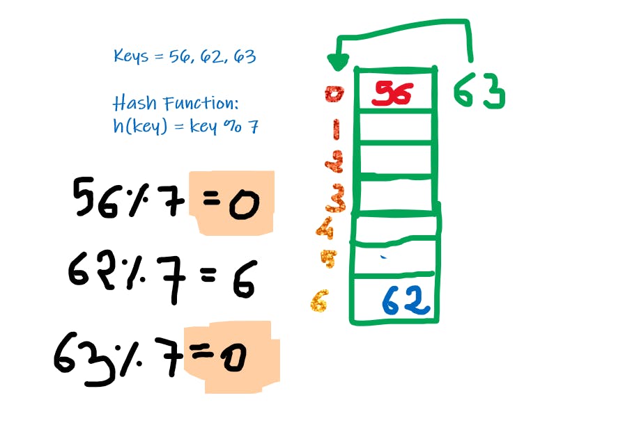
Collision Prevention Techniques:

1. Chaining

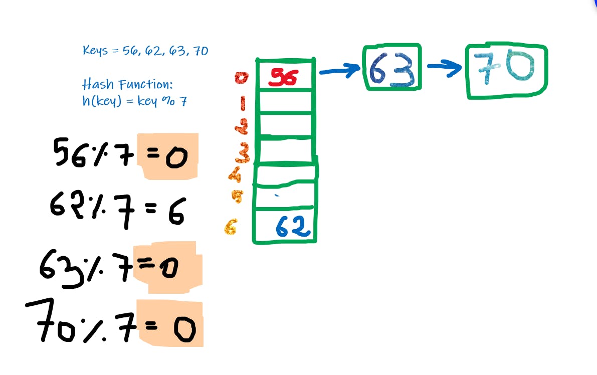
• Here instead of array (normal), we maintain Array of Linked List Heads, Hence if we get the same values, we just connect them via Linked List on the same index which creates a sort of chain-like structure.
• Below illustration demonstrates Chaining:

Performance Analysis of Chaining:

Let's assume
    m = Number of slots in the hash table
    n = Number of keys to be inserted

Load Factor (α) can be denoted as n/m

If we assume uniform distribution of keys among hash table then:
    Expected Chain Length = α
    Expected Time to Search = O(1 + α)
    Expected Time to Insert/Delete = O(1 + α)

Hence for uniform distribution on average, α can be equated as 1 
    Expected Chain Length = 1
    Expected Time to Search = O(1)
    Expected Time to Insert/Delete = O(1)

Algorithms for Search, Insert, and Delete in Chaining:

function Insert(int keys) {
    i = key % (size of Hash Table)
    table[i].push_back(key)
}

function Delete(int keys){
    i = key % (size of Hash Table)
    table[i].remove(key)
}

function Search(int keys){
    i = key % (size of Hash Table)
    for(auto x in table[i])
        if(x == key)
            return true
    return false
}

Data Structures used for Chaining:

1. Linked Lists:

• All the three operations namely Search, Insert, and Delete will take O(l) time where l is the length of the linked list. Also linked lists are not cache friendly.

2. Dynamic Sized Arrays (Vectors, ArrayLists):

• All the three operations namely Search, Insert, and Delete will take O(l) time where l is the length of the linked list. But they are also cache friendly.

3. Self Balancing Binary Search Trees (AVL Tree, Red-Black Trees):

• All the three operations namely Search, Insert, and Delete will take O(log(l)) time where l is the length of the linked list. But they are not cache friendly.

Advantages:

1. Pretty straightforward to implement
2. As Linked Lists are dynamic, we can add more and more elements to it
3. Robust against load factors or hash functions
4. It's mostly used when we don't know the number of keys we have to add

Disadvantages:

1. As Linked lists are not cached friendly, overall performance gets impacted
2. If every key has the same index then for n elements, chain length becomes n, hence the search time will become O(n)
3. Space also gets occupied unnecessarily

2. Open Addressing:

Introduction:

• Like Chaining, Open Addressing is a Collision Handling technique in which we only use a single array (1 Hash Table only) to store all the keys. To achieve this, some points must be remembered:
  1. Number of Slots in Hash Table >= Number of keys to be inserted
  2. It is Cache Friendly as we are using arrays

Performance of Open Addressing:

Let's assume
    m = Number of slots in the hash table
    n = Number of keys to be inserted

Load Factor (α) can be denoted as n/m will be less than 1

If we assume uniform distribution of keys among hash table then:

    Expected Time to Search = O(1 / (1 + α))
    Expected Time to Insert/Delete = O(1 / (1 + α))

Types of Open Addressing:

1. Linear Probing:

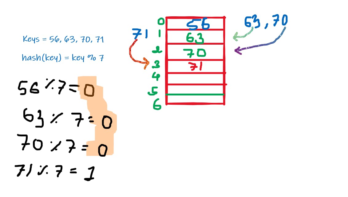
Introduction:

• In linear probing, we search for the next empty index whenever we have a collision
• Few points to be noted about Search and Delete operations:
  1. Search:
     • We compute the hash function, and we go to the index, and compare. If we find the element we return it otherwise we linearly search and only stop when:
       1. We encounter an empty slot
       2. The key need to be searched is found
       3. We have traversed through the entire array
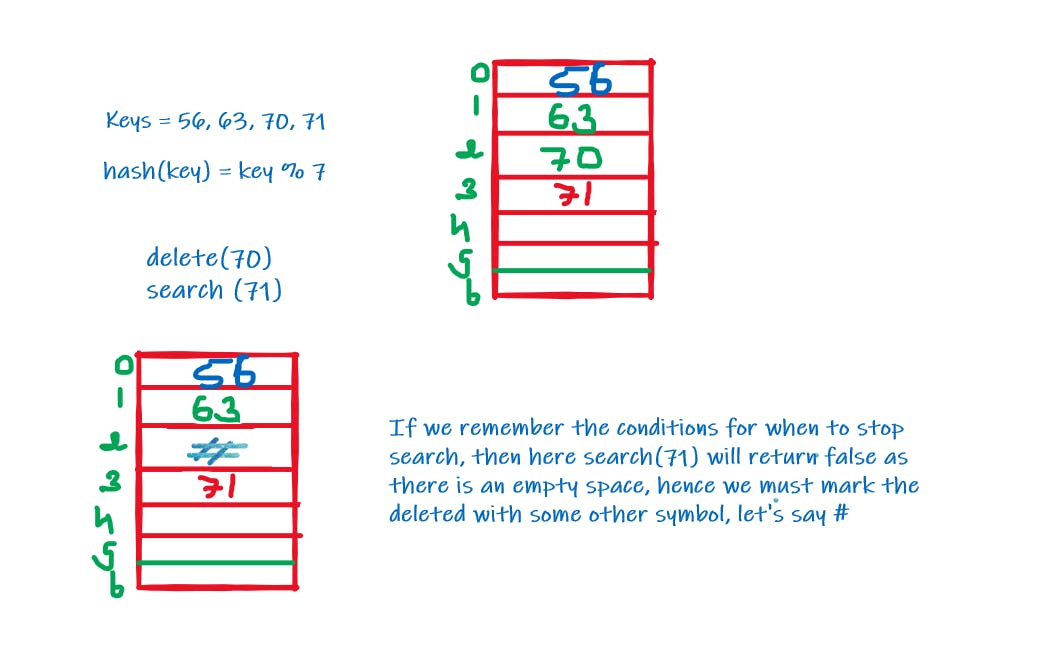
  2. Delete:
     • One thing to remember is that we cannot just simply remove the key from the index as it may cause search failure, instead we mark the slot with some other symbol to ensure nothing gets broken and the element also gets deleted.

Challenges:

1. Primary Clustering: One of the problems with linear probing is Primary clustering, many consecutive elements form groups and it starts taking time to find a free slot or to search for an element.
2. Secondary Clustering: Secondary clustering is less severe, two records only have the same collision chain (Probe Sequence) if their initial position is the same.

To overcome these challenges, we use Quadratic Probing.

2. Quadratic Probing:

Inroduction:

• The hash function in this probing looks like:

  hash(key, i) = (h(key) + i²) % m

• Here initially we start from the original location (i=0), if we have a collision we try a value of i=1 then 2,3.... till we encounter an empty slot.
• Quadratic Chaining is guaranteed to work when:
  • α (Load Factor) < 0.5
  • m is prime

Challenges:

• Problem of secondary clustering prevails

3. Double Hashing:

Introduction:

• The hash function in this probing looks like this:

  hash(key, i) = (h1(key) + ih2(key)) % m

• Initially, we strive for the original position (i=0), if we have a collision, then we look for i=1 then 2,3, and so on...
• If h2(key) is relatively prime to m, then it always finds a free slot if there is one
• Distributes keys more uniformly than Linear Probing and Quadratic Probing.
• No Clustering happens, neither primary nor secondary